This shows how to parameterize dipfk for velocity filtering using modelling and display tools
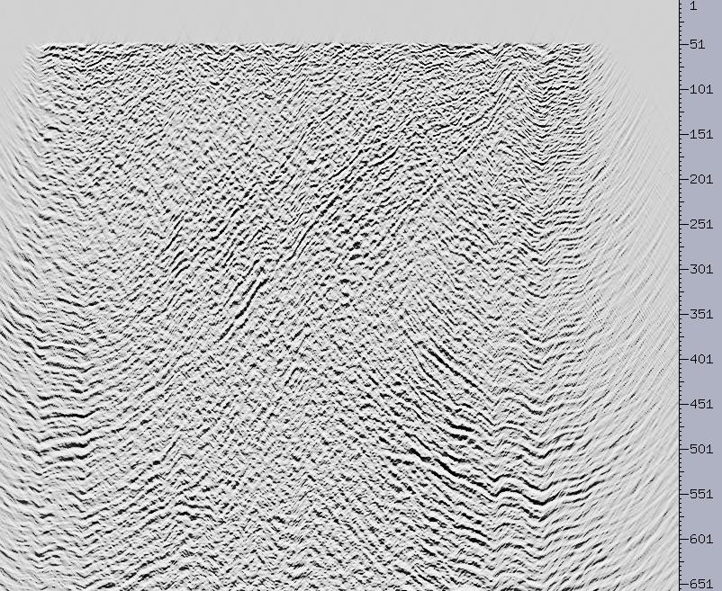
Input offset xsd display of record off10
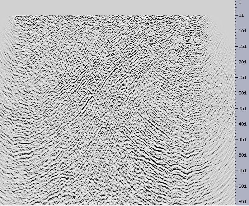
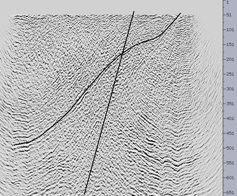
Input offset with xsd picks illustrating geology and noise. The
steeply dipping event is noise.
The picks are saved in xsd using File -> Save Segments and then supplying
a file name (ich_pik)
and sample units (in this case 10)
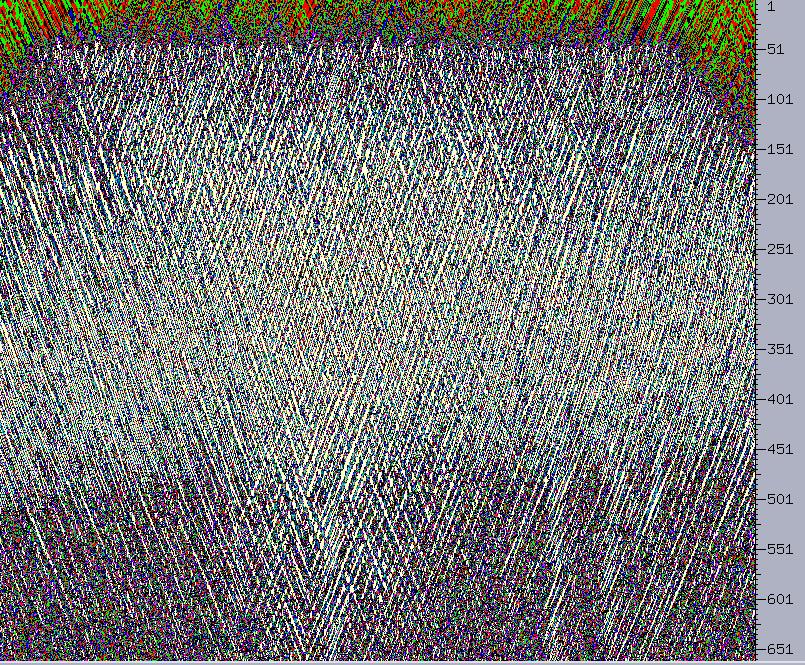
The result of running
ich -N off10 -P ich_pik -S | filt -O ich_rec -fl .1 -fh 12 -nor
4 -M
You get a record with exactly the geometry of the input data but with
only the events you picked. This is a very quick and easy poor man's modelling
approach excellent for tracking events through transform space.
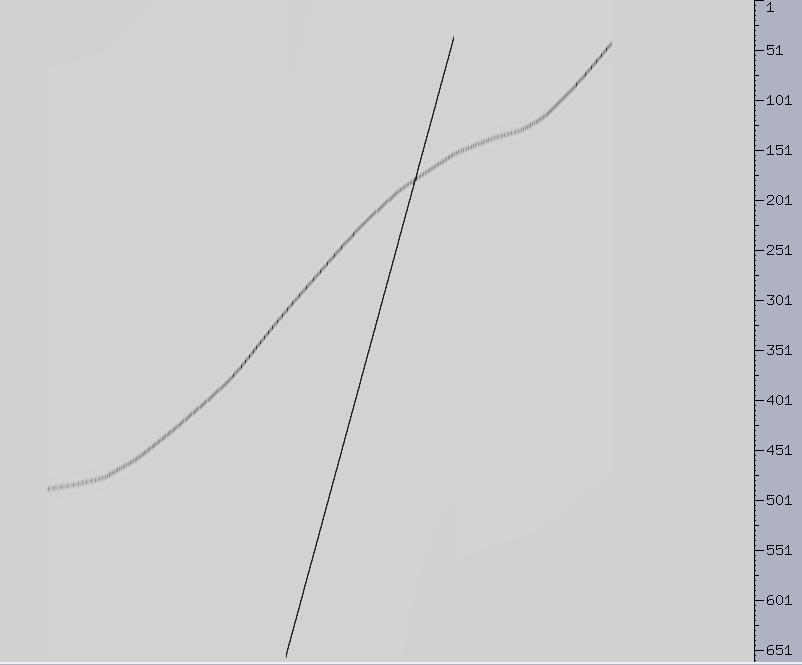
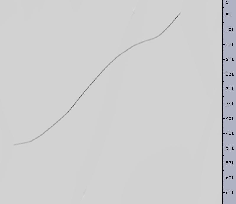
Here is the xsd pick segment for the low velocity event
Segment = 2 Name NO_PICK_NAME_HERE
color = -43 picks = 2
1.000000 287.000000 6560.000000
1.000000 455.000000
370.000000
The trace units (column 2) are 20 and the time units (column 3) are
already
in place. So to compute the velocity we simple do the following:
(455 - 287 - 1) * 20 = 3340 [horizontal distance]
6560 - 370 = 6190 [vertical "time"]
velocity = 3340/6.19 = 540 m/s
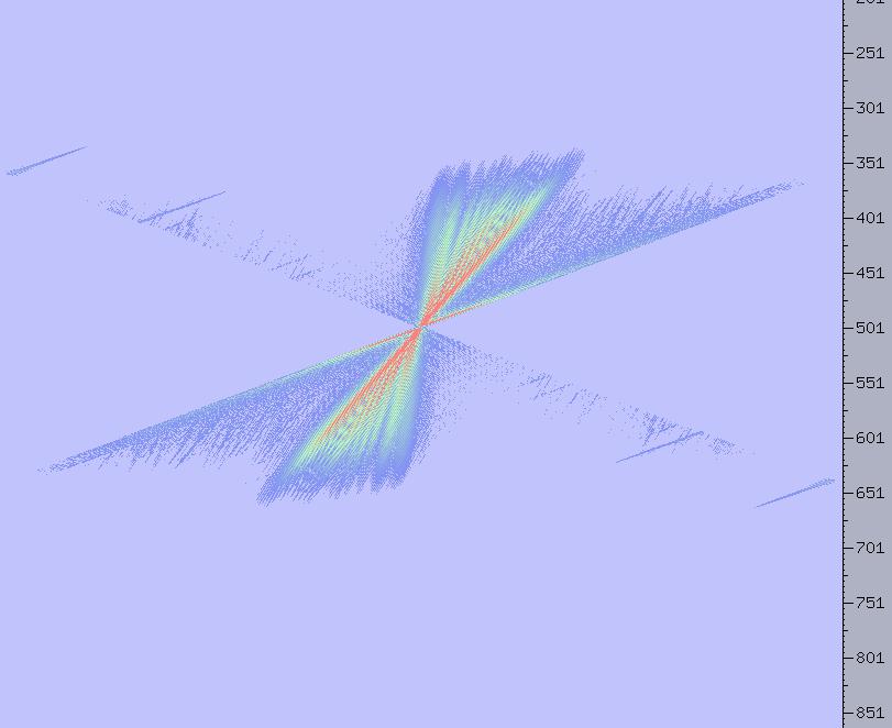
Display of the top half of the record from running
fftxy -N ich_rec -O ich_reckk

The origin is located in the center of the plot. The vertical axis
is "temporal" frequency and the horizontal axis is spatial frequency.
The unit spacing of the vertical axis is half that of the horizontal axis
so the slpoe of the low velocity event is about the same as calculated
above.
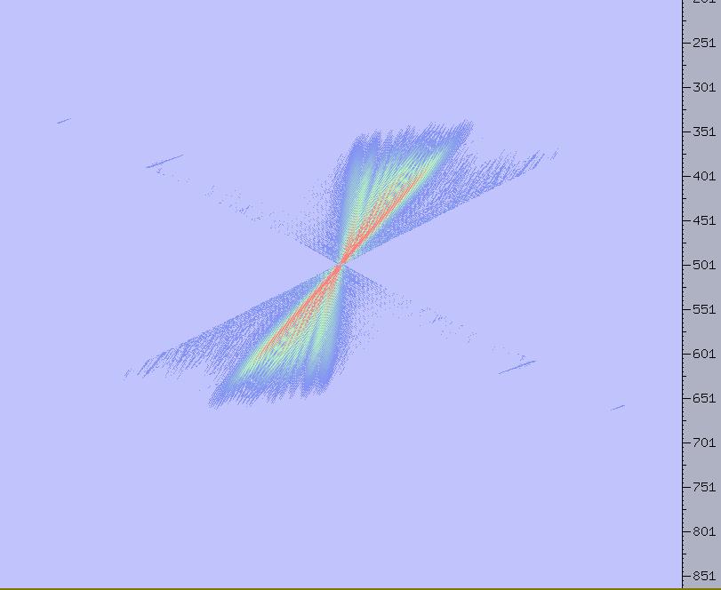
The result of running dipfk -N ich_reckk -O ich_reckkdipfk -vs-600
-ve600 -dx20 -P on the KxKy record above. The pie shaped wedge is
clearly visible and does not successfully mute the low velocity event.
Let's try dipfk -Nich_reckk -Oich_reckkdipfk -vs-800 -ve800 -P -dx20
on the KxKy record. Look, the wedge now mutes the low velocity event
but leaves the "geology" alone.
Now we run the inverse transform fftxy -N ich_reckkdipfk -O ich_reckkdipfkR
-R to get the image below. Note that we have successfully removed
the desired event (there is a little transform noise from the ends of the
event but that won't impact our methodology).
We can now take these parameters and apply them to our offset record
Taking the difference of the input offset record and the filtered off set record and display at a boosted amplitude scale we get
For 3D the approach is basically the same. The analysis will have to be done on both an inline and a crossline cut through the offset volume. After the velocity ranges are determined then the flow will look something like
fftpack ... |\ #time -> temporal frequency
ttds3d -NDtxy -ODxyt |\ #frequency slices
vfilt3d ... |\ #velocity filter
ttds3d -NDxyt -ODtxy |\ # back to frequency orientation
fftpack -R |\ #frequency -> time
hdrswap -N2 [input data] -O [output data] #swap in headers
from input data
