Upscaling Petrophysical Properties to the Seismic Scale
Upscaling Petrophysical Properties to the Seismic Scale
Greg A. Partyka, Jack B. Thomas, and Kevin P. Turco, BP
Dan J. Hartmann, DJH Energy Consulting
Previously published by the SEG in: Extended Abstracts of the 2000 Exposition and Seventieth Annual Meeting of the Society of Exploration Geophysicists, Calgary, Canada.
Summary
Seismic measurements respond to reservoir/petrophysical properties at a larger scale (i.e. seismic wavelet scale) than well-log or core measurements. Determining whether seismic can delineate variability in petrophysical properties therefore requires scoping work that tackles scale of measurement issues. Backus filtering provides one such method for upscaling well-log based measurements to the seismic scale.
Introduction
Our ability to make precise, timely, and cost effective business decisions during field development, is largely based on the quality of technical information. Operations are expensive, and we often look to seismic to determine the extent and quality of the target reservoir unit(s). To play a key role in reservoir definition, seismic requires calibration to petrophysical properties.
Use of 3-D seismic has revolutionized the geophysicists' ability to spatially map reservoir targets. In many cases however, seismic falls short in quantifying petrophysical variability; its use often extending only as far as mapping spatial patterns that help the geologist establish the structural and stratigraphic setting. If petrophysical reservoir characteristics can be estimated "pre-drill" with confidence, early reservoir simulations can help with proper sizing of production facilities and drilling costs.
When structural or stratigraphic patterns are exposed, there is a large (typically unrealistic) temptation to infer petrophysical reservoir models directly from bandlimited seismic scale maps and volumes. The path from core data to seismic data to reservoir flow-modeling requires understanding of the interplay between flow-unit stacking, thickness, velocity, and bandwidth. Such understanding enables the interpreter to answer two basic questions: such as:
1. Does seismic respond to the variability in petrophysical properties?
2. What scale of petrophysical variability can be resolved with what seismic bandwidth?
Engineering design estimates from these data should only be done after rock-to-log-to-seismic calibration has been completed.
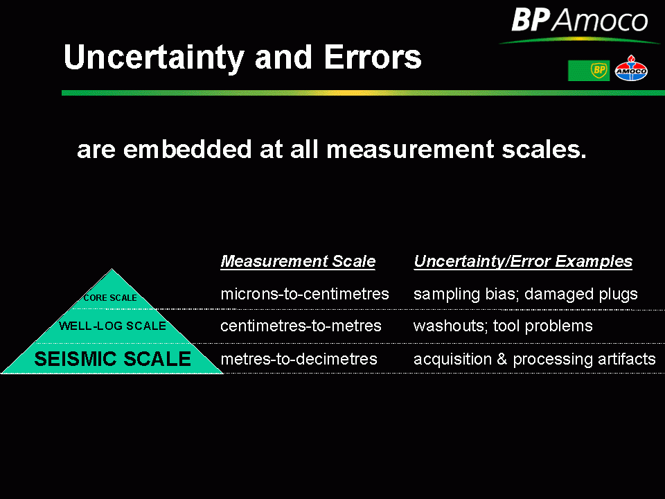
A great deal of uncertainty is imbedded in seismic-petrophysics calibrations because of large variations in scale of measurements. Core analyses provide information on the micron to centimetre scale; well-logs on the centimetre to metre scale, seismic on the metre to decimetre scale. In addition to these upscaling and downscaling issues, the individual datasets can contain errors such as:
Sampling bias and sampling induced damage to core plugs,
Washouts,
Tool problems in well-log measurements,
Acquisition and processing artifacts that mask the true seismic response from the reservoir.
Determining qualitative gross reservoir geometries from seismic can be relatively straight-forward and fast, but may contain large uncertainties. Determining whether seismic can delineate variability in petrophysical properties however, requires scoping work on a finer level that tackles scaling issues. One such scoping approach can be broken down into two steps:
Step #1: Cross-Plot well-log-scale acoustic properties versus petrophysical properties. Do well-log scale crossplots indicate acoustic sensitivity to petrophysical properties? If yes,...there is hope for seismic; if no,... seismic will not add value to mapping petrophysical variability.
Step #2: Perform upscaling sensitivity analysis with respect to bandwidth, flow-unit thickness, velocity and flow-unit stacking; then use derived relationships to transform seismic inversion-derived acoustic properties to petrophysical properties.
Step #1: Scoping at the Well-Log Scale
A good starting point is to look at data from key wells that are petrophysically characterized and contain acoustic log measurements (compressional sonic, shear sonic and density). In step #1, crossplot well-log based acoustic measures such as acoustic impedance and Vp-Vs ratio versus calibrated well-log derived petrophysical properties such as water saturation, volume of shale or porosity. Such simple cross-plots ignore up/down scaling (seismic bandwidth) issues and provide a best case (well-log scale) scenario for the resolving power of seismic with respect to petrophysical delineation. If the acoustic measurements exhibit no sensitivity to petrophysical properties at this seismically unrealistic well-log scale, the game is over; bandlimited seismic will provide little value in inferring petrophysical reservoir variability. If however, well-log scale acoustic data discriminates the petrophysical properties of interest, the game continues to step #2: understanding up/downscaling issues.
At the end of step #1, the interpreter has two pieces of information in hand:
1. Seismic data derived acoustic volumes and maps of the reservoir interval, and
2. Well-log scale crossplots between acoustic and petrophysical properties.
Step #2: Sensitivity Analysis for Upscaling
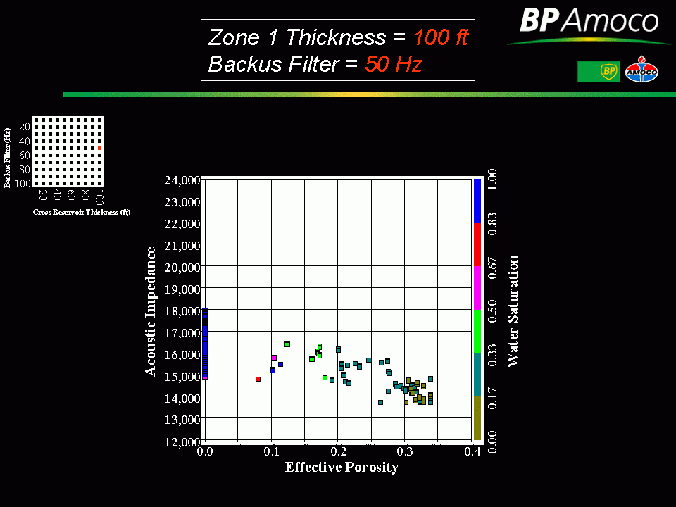
With well-log-scale data in hand from step #1, it is tempting to establish acoustic-petrophysical relationships at the well-log scale, then directly apply them to the acoustic impedance data derived from bandlimited seismic, and determine spatial variations in petrophysical properties. That approach however, does not address the scale differences between the two sets of data, and may provide erroneous reservoir characteristics. As we scale up (or bandlimit) the acoustic measurements, the acoustic resolving ability becomes a moving target that is dependent on four criteria: thickness, velocity, bandwidth and flow-unit stacking. The shape of the best line fit through the acoustic-petrophysics cross-plots changes with any change in the criteria. An acoustic impedance value can represent a range of possible petrophysical values (e.g. porosities) depending on local thickness, velocity or flow-unit stacking.
We recommend upscaling the acoustic measurements using a range of upper frequency cut-offs. This enables a sensitivity analysis of upper frequency versus petrophysical resolving power, for one particular flow-unit stacking pattern and thickness. Simply filtering a well-log interval with various hi-cut filters deals with only the frequency upscaling part of the sensitivity problem, and disregards the remaining three criteria of the upscaling sensitivity matrix (flow unit stacking pattern, thickness and velocity). Quantifying seismic resolution requires a sensitivity analysis with respect to all four criteria. In other words, Backus-averaging only one well-log-based zone of interest does not uniquely determine the resolving power of a particular seismic bandwidth with respect to petrophysical properties for all other thicknesses. It does so, only for the one particular vertical thickness and the one particular ordering of layers inherent in the well-log profile. If the thickness or stacking order of individual layers changes, the resolving power of the seismic bandwidth with respect to petrophysical properties will also change. For exampe, if you progressively decrease the wavelet bandwidth (i.e. hi-cut frequency), you also progressively decrease the resolving ability of impedance with respect to porosity. Note that by the time you cut-back the frequency to 30hz, the acoustic impedance-versus porosity relationship is relatively flat, indicating that it would be very difficult to quantify porosity variability in a 50ft bed using 30hz signal. There remains however, a contrast between porous-oil-filled sand and the shale, indicating that detection of porous sand (in a 50ft bed, using 30hz signal) is still possible. You can create a similar effect by maintaining the same bandwidth while progressively decreasing thickness. To assess the ability of bandlimited seismic to resolve the range of flow unit thicknesses and stacking patterns:
1. Establish end-member flow unit profiles (the expected range of flow unit stacking orders and flow unit thicknesses), then
2. Backus-average each model with a range of upper frequency cut-offs.
The well-log scale cross-plots created in step #1, that were used to determine whether seismic can discriminate petrophysical variability, should then be replotted; one crossplot per combination of:
Flow-unit thickness,
Flow-unit velocity,
Flow-unit stacking-pattern, and
Frequency hi-cut,
for the entire realistic range of these four variables. This kind of upscaling sensitivity analysis quantifies the ability of seismic to characterize petrophysical variability with respect to the four variables. In effect, this kind of scoping work is the seismic-petrophysics equivalent of a seismic upsum filter analysis, except for one big difference: conventional upsum filter analysis indicates resolution with respect to wavelength. This analysis on the other hand, indicates resolution with respect to petrophysical properties.
Step #3: Predicting Petrophysical Properties from Seismic Impedance
Predict petrophysical properties from seismic impedance requires knowledge of:
the seismic wavelet, which can be obtained via conventional spectral analysis,
seismic-derived impedance, which can be obtained via seismic inversion techniques,
upscaling sensitivity relationships, from step #2 above, and
gross thickness.
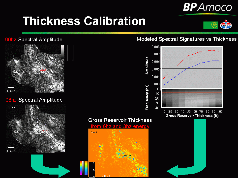
One way to derive gross thickness is via:
computing a spectral decomposition Tuning Cube for the zone-of-interest,
thickness modeling to derive local energy-vs-thickness-vs-frequency relationships, and
interpreting a guide horizon along the zone-of-interest,
subsetting a short, zone-of-interest volume,
computing a zone-of-interest Tuning Cube (i.e. computing an amplitude spectrum for each time-trace), and
animating vertically (in plan view) through the Tuning Cube to examine reservoir tuning effects.
This Tuning Cube, in plan view, allows you to examine reservoir zone amplitude maps at any frequency, thereby revealing structural and stratigraphic details.
To derive local energy-vs-thickness-vs-frequency relationships, create a wedge model for the reservoir by stretching/squeezing the well-log reservoir zone to simulate a variety of thicknesses (e.g. from 10 to 100 feet in increments of 10 feet); then compute the spectral decomposition for the wedge model, in the same manner as for the real data. At this stage you have the necessary information to calibrate the real Tuning Cube with the modeled estimates.
From the modeling you can determine the frequency below which the entire thickness range stays below resolution. Staying below resolution allows you to uniquely associate a thickness with each amplitude. If you cross-over to higher frequencies, part of the possible thickness range becomes resolved, and you will no longer be able to uniquely asociate a thickness with amplitude (i.e. the amplitude versus thickness relationship would turn over itself. So, proceeding with a low-frequency component enables less-subjective gross thickness estimation.
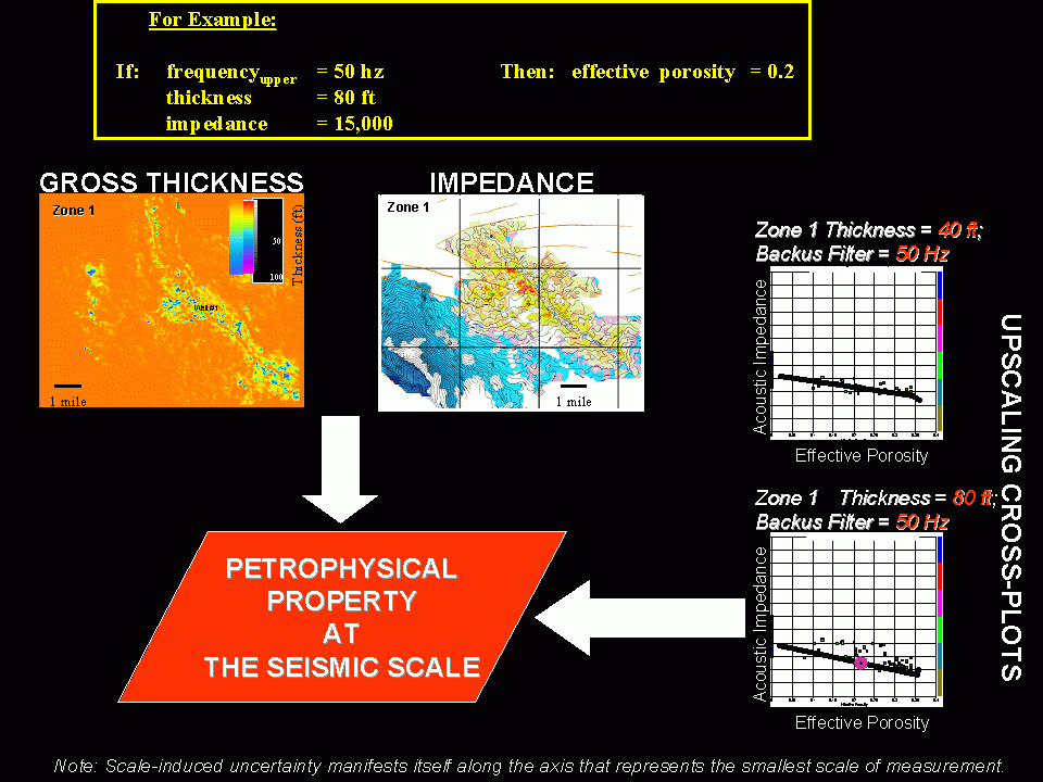
At this stage you have all the necessary pieces to predict petrophysical properties from the seismic. The gross thickness and wavelet hi-cut frequency determine which upscaling-sensitivity cross-plot to use.
Conclusions
The procedure outlined here, allows interpreters to examine acoustic-petrophysics relationships at the seismic scale. The resulting relationships can be used to transform seismic inversion-derived acoustic properties to petrophysical properties. This allows using more realistic, appropriately complex reservoir models that take into account reservoir thickness and flow-unit stacking. Using this method, models can be built that reflect what the rock system truly looks like at the seismic scale.
References
Backus, E.B., Long-Wave Elastic Anisotropy Produced by Horizontal Layering, Journal of Geophysical Research, vol. 67, no. 11, 4427-4440, 1962.
 Return to Online Training