Seismic Thickness Estimation: Three Approaches - Pros and Cons
Greg Partyka, bp
1998
Previously published by the SEG in: Extended Abstracts of the 2001 Exposition and Seventy First Annual Meeting of the Society of Exploration Geophysicists, San Antonio, U.S.A.
Summary
Spectral decomposition provides a robust and phase-independent approach to seismic thickness estimation. It builds on traditional tuning thickness estimation techniques documented by Widess (1973) and Kallweit & Wood (1982). Whereas these traditional techniques require zero-phase data and careful picking of temporally adjacent peaks and troughs, thickness estimates derived from spectral-decomposition-derived discrete Fourier components are wavelet-phase independent and require only one guide pick within the seismic zone of interest.
Introduction
A simple wedge model was used to illustrate, compare and contrast three techniques for seismic thickness estimation:
Of the three methods, thickness via discrete Fourier components provides the most robust and least labour-intensive approach to seismic thickness estimation.
Model Data
The wedge model that was used to illustrate and compare the thickness estimation methods consists of 50 traces, 250 milliseconds in length. The top of the wedge is at time 100ms. The wedge thickens from 0 ms on the left to 50 ms on the right. Each trace contains two reflectivity spikes of equal amplitude but opposite sign. The top spike is located at the top of the wedge. The bottom spike is located at the bottom of the wedge. To model sub-resolution thickness, the model was filtered with a zero-phase 8-10-40-50 Hz Ormsby filter.
Approach 1: Conventional Tuning Thickness Analysis
This first approach is based on work performed by Widess (1973) and Kallweit & Wood (1982), and requires careful mapping of peak-trough time separation as well as careful mapping of amplitude variability. Accurate thickness predictions depend on accurate seismic processing to establish the correct wavelet phase. Valid thickness estimates will prevail only if the seismic data is truly zero-phase and trace-to-trace amplitudes are preserved. Below the tuning thickness limit (Ttu), amplitude varies as a function of thickness variation (as long as the entire amplitude variation is caused by tuning effects). Above the tuning thickness limit (Ttu), the top and base of the bed are temporally resolved, and thus the peak-to-trough time separation can be used to map thickness variability.
Because this method requires careful event picking and quality control, it often results in more hands-on time by the interpreter. It requires two attributes (i.e. two mapped events) to quantify thickness:
1. Peak-trough time separation for thickness greater than the tuning-thickness (Ttu), and
2. Amplitude for thickness less than the tuning-thickness (Ttu).
Approach 2: Dominant Frequency and Dominant Amplitude Mapping
This method stems from the spectral decomposition tuning-cube approach to thickness mapping. By spectrally decomposing the seismic data into the frequency domain via the discrete Fourier transform (DFT), the amplitude spectra delineate temporal bed thickness. While the tuning-cube as a whole characterizes the zone-of-interest rock mass variability, interpreting geophysicists prefer if possible, to boil the tuning-cube information down to one or two maps. One approach to such consolidation is to pick the first dominant frequency and create two maps:
In thickness mapping, these dominant amplitude and dominant frequency maps are analogous to the time separation and amplitude maps of approach-1. For thicknesses less than the tuning thickness (Ttu) limit, dominant amplitude information encodes the thickness variations (provided the entire energy variation is caused by tuning effects). For thickness greater than the tuning thickness (Ttu) limit, dominant frequency encodes thickness variability (provided the entire energy variation is caused by tuning effects). Both the dominant frequency and dominant amplitude are required to characterize the thickness range. Beyond a threshold thickness (Tth) related to the hi-cut frequency however, neither dominant frequency nor dominant amplitude is able to quantify thickness.
This method provides two advantages over the traditional methods: phase independence and the requirement of only one guide pick within the seismic zone of interest to guide the spectral decomposition analysis window. However, as in the traditional approach, two attributes are required to quantify thickness:
1. Dominant frequency for thickness greater than the tuning thickness (Ttu), and
2. Dominant amplitude for thickness less than the tuning thickness (Ttu).
Approach 3: Thickness via Discrete Fourier Components
Rather than extracting the peak frequency and peak amplitude from the spectral decomposition tuning-cube, thickness can be derived from amplitudes extracted at discrete Fourier components. Though similar in context to traditional methods, this spectral method once again uses a more robust phase independent amplitude spectrum and is designed for examining thin bed responses spanning large 3D surveys. Here, the value of the frequency component determines the period of the notches in the amplitude spectrum with respect to thin bed thickness:
Pt = 1/f
Where:
Pt = Period of notches in the amplitude spectrum with respect to temporal thickness (seconds), and
f = Discrete Fourier frequency
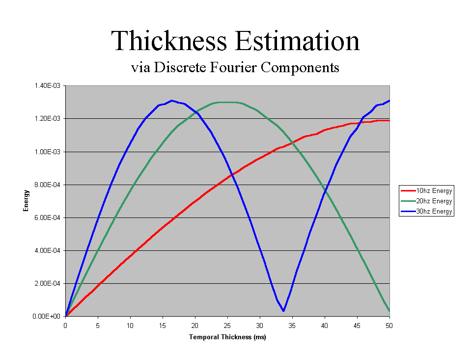
Each thickness/velocity/frequency combination exhibits a characteristic relationship. Even a relatively low frequency component such as ten hertz quantifies thin-bed variability. In fact, by choosing appropriately low frequency components, the entire range of possible thickness is forced below the tuning thickness (Ttu), and can therefore be quantified using a single attribute: amplitude variability. Removing the need for dominant frequency simplifies the analysis.
If desired, the low-frequency-derived thickness can be refined by introducing progressively higher frequencies into the calibration. For example, examine the discrete Fourier components. Amplitude=0.0004 at 10hz indicates a 10ms two-way-time. Amplitude=0.0008 at 20hz however, used in isolation, indicates two possible two-way-times: 10ms or 40ms. Thickness from the 10hz however, can be used to define the relevant portion of the 20hz amplitude curve, thereby revealing a unique 10ms two-way-time at 20hz.
If signal to noise ratio is a problem, this method allows the interpreter to selectively choose and analyze those frequencies exhibiting highest signal-to-noise ratios. As in approach-2, only one picked horizon is required within the seismic zone of interest to guide the spectral decomposition analysis window. As with the other two methods, complex flow-unit distributions require careful seismic modeling and spectral decomposition analysis to determine relationship between spectral response and thickness.
Conclusions
The Spectral Decomposition method provides a robust and phase-independent approach to seismic thickness estimation. Although similar in concept to the traditional techniques documented by Widess (1973) and Kallweit & Wood (1982), the spectral decomposition technique requires only one analysis-guide-pick for the analysis window rather than the traditional careful picking of adjacent peaks and troughs. By using approach-3 (thickness via discrete Fourier components) and appropriately low discrete frequencies, the entire range of expected thicknesses falls below the tuning thickness (Ttu). By forcing all thickness to fall below the tuning thickness, thickness can be inferred directly from energy alone.
References
Widess, M.B., 1973, How Thin is a Thin Bed?, Geophysics, vol. 38, pg 1176-1180.
Kallweitt, R.S. and Wood, L.C, 1982, The Limits of Resolution of Zero-Phase Wavelets, Geophysics, vol.47, pg 1035-1046.
Partyka, G.A., Gridley, J.M., and Lopez, J. 1999, Interpretational Applications of Spectral Decomposition in Reservoir Characterization, The Leading Edge, vol. 18, No. 3, pg 353-360.
PowerPoint 2000 Version of this material.
 Return to Online Training