
This tutorial is being developed on the fly with interested FreeUSP users. If there is something you would like covered in this section please post to freeusplist@freeusp.org and we will see if we can include it. This is a work in progress and will progress as user demand and my ability to apportion time to the exersize dictates. Also, when I get a few hours to pound out a new section I am moving pretty fast. If you see me come off the rails, please chime in. The faster we correct any mistakes, the better for everyone involved....Paul G. A. Garossino
Corrections and contributions from:
Fernando M. Roxo da Motta [Dec 15, 2005]
 Residual Statics
OK, let's get started. The goal here is to take a dataset from SEG-Y data as might be obtained from a contractor and get to a stacked image useful for interpretation. I don't know what kind of disaster I am letting myself in for here, but what better way to stress a toolkit than process a line submitted by the user community live fire. Who wants to supply the guinea pig line? Anyone?
Waldek Ogonowski (Ray) has done us the great favour of making available a land vibroseis dataset donated to the public domain by Geofizyka Torun Sp z o.o, Poland. Thanks very much Ray!
Once you have the data on disk your directory should look something like:
-rw-r--r--    1 zpgg07   techgrp       866 2005-02-18 12:59 Line_001.TXT
-rw-r--r--    1 zpgg07   techgrp     21951 2005-02-18 13:00 Line_001.XPS
-rw-r--r--    1 zpgg07   techgrp     21951 2005-02-18 13:00 Line_001.SPS
-rw-r--r--    1 zpgg07   techgrp     64962 2005-02-18 13:00 Line_001.RPS
-rw-r--r--    1 zpgg07   techgrp  445100896 2005-02-18 14:04 Line_001.sgy
Fire up xsd [ X Seismic Display] which is the FreeUSP seismic viewer. To do this simply type:
xsd &on the command line. If your system is installed correctly you will shortly see the xsd mother window appear on your screen.
If this is your first exposure to the tool you should be aware that xsd is a client/server application. The client program runs on your local machine and allows for display and interaction with your data. The server program runs on any host computer that you specify. The server rasterizes the data for display and supplies a compressed version of that rasterization back to the client program for display. This allows one to efficiently view data from remote locations. If you only have one machine then the client and server will both be running on your local box.
xsd can display many formats of data including USP, DDS, man flavours of SEG-Y, many flavours of binary cube and SEP.
Download the xsd colourmaps and install them in a directory under your home. You can name that directory anything you want so why not use Colourmaps.
You can, and eventually will, create you own colourmap files anytime you want. For this tutorial however it will be useful for us all to use the same colourmap when conversing about any aspect of the data.
Prior to plotting your first bit of data click on the Options entry on the mother window. From the options pull down menu detect Project. The Project File window that appears allows you to set some global parameters. Fill out the entries indicated with values appropriate for your installation. The = entry next to Host Computer causes the server to start up on the local machine by default. Detect Save as Default once you have made your entries. xsd will create a .xsd_defaults file on your home directory to store these defaults in.
Now click on File on the xsd mother window. You will see a Server Startup window appear. If your data is on your local machine then simply hit OK. If not then fill out the appropriate hostname in the Host Computer area first.
You will not see this menu again for the remainder of this session. If you ever need to restart the server on another machine you will have to detect the Restart Server entry on the File pull down menu.
After you hit OK you should see a Seismic File window appear. If you have not entered the Directory name where your data is stored you can do so now. You will see a list of all the files present in that directory in the Files area of the display. Turn off the Automagically recognize the seismic format button and double click [left mouse button] on Line_001.sgy. You should see the Seismic Data Format window appear. Scroll down to segy and double click.
The Server Parameters window should now be on the screen. Notice that since there is no entry in the SEG-Y world for the number of records in the dataset xsd has defaulted to a very large number. So the program thinks there are some unknown number of single trace records in the Line-001.sgy file. We know that there should be 251 records and that, including the auxillary channels, there should be 284 traces per record.
Fill out the Server Parameters menu as indicated and hit OK.
We are going to take a look at the first 1000 traces of the SEG-Y dataset. We just want to see what we are up against data-wise. Notice that I have used a maximum scalar of 2 and a scaling exponent of 2. This will cause a t2 scaling to be applied which is likely necessary as this is raw unscaled data. Also be sure to use the gray4 colourmap at this time.
The resulting display is nearly blank except for some very high amplitude arrivals on one of the auxillary traces. If you crank up the contrast you will start to make out the outline of the data traces. Since we have such a large amplitude range, and given that we are not really doing data QC at this point, I am going to switch from using a maximum scalar to using a Range Histogram scalar. Notice that I can no longer identify outlier amplitudes but at least I can see the nature of the data. I looks like we have valid data in the SEG-Y file.
Feel free to experiment with xsd by plotting different chunks of the input data. You will soon have many windows on the screen. xsd has a facility to manage all those windows. At any time you can click on the Window pull down menu of any display window. Detect Hide and that window will disappear from the screen. If you have many windows up and don't want to have to hit Window and Hide on every window you can bring up the Global window by clicking on the Global entry of the Window pull down menu. You can also use the acceleration keys for many of these actions. For instance, if you hit Alt-g while your focus is on a display window the Global window will appear. If this doesn't happen for you, make sure your Num Lock is off. You will also notice that the acceleration keystrokes associated with any give menu option are listed to the right of the item on the xsd menues.
With the Global window up you will see everything that you have plotted so far listed in the window list. If you double click on any entry there it will appear in the selected window area below. Once you have selected the entries you desire you can there cause all kinds of things to happen using the buttons at the bottom of the menu. For right now just hit Hide. The difference between Hide and simply iconifying the window is that hidden windows are swapped out of active memory. Iconified windows are not. As you plot a pile of stuff over the course of a day you may get into serious trouble with memory unless you get used to using the Hide facility of xsd.
FreeUSP routines read data in USP format. USP format is a grandfathered version of AMOCO's original SIS [Seismic Information System] tape format which was in use when digital seismic data processing grew up inside the company. A USP dataset starts with a line header containing information global to the dataset such as sample integerval, total number of records, traces per record, samples per trace and the like. Near the end of the line header is an historical line header [hlh] which contains the processing history of the dataset. After the line header comes the traces. Each trace is made up of a trace header and a trace data series. The trace header contains information pertinent to that trace such as source position, receiver position, trace distance and the like. All line and trace header entries are defined by mnemonic so that the user doesn't have to know anything about the actual byte format of either in order to make header entries and modifications. The mnemonic definitions are maintained in the low level development libraries behind the scenes so that changes can be made from time to time without affecting the user's perception of the format.
We have also created mnemonic definitions for all SEG-Y reel header and trace header entries. This allows the user to easily create mapping files between the two formats without detailed knowledge of byte format descriptions.
To get a complete description of both format [and others] simply type:
hdrdesc
If you would like to capture the output try typing:
hdrdesc | xcat -menuwhich will pipe the output of hdrdesc into an xcat scrollable window. You may file the stuff away or simply dismiss the window when you are finished with it. xcat is an X11 version of the UNIX command cat. The routine was written by Joe Wade, Phil Fincannon and Steve Farmer years ago at Amoco Tulsa Research and has been a gold standard on the UNIX command line every since. Check out it's capabilities at any time [as you can of any FreeUSP routine] by typing:
uman xcatOK, now to get down to business. In FreeUSP there are three routines basic to conversion between SEG-Y and USP formats. These are segy2usp, usp2segy and the FreeDDS routine bridge. Each has its advantages depending what you are up to and we will be using usp2segy and bridge here as part of the tutorial.
Data format conversion requires a detailed knowledge of two things about the input SEG-Y data; what header entries are valid and what flavour of SEG-Y format are we dealing with. Almost all data floating around out there in SEG-Y format is in what I will call "classic" SEG-Y format. That is more or less the 1975 standard. I have recently seen my very first SEG-Y dataset in the SEG's revised format which I will call the "new" SEG-Y format. The SEG-Y format description utilized by segy2usp and usp2segy is the "classic" format. bridge on the other hand can deal with either "classic", the default, or "new" SEG-Y format as defined by the in_format= entry on the command line. I notice that at the moment the version of bridge in FreeDDS defaults to the "new" SEG-Y format. We have changed this in house as it caused too many problem with the majority of our SEG-Y data which utilized the spare area from bytes 180 to 240 of the traces headers to store indexing. I am pretty certain that Jerry Ehlers will shortly be updating the FreeUSP version of bridge to stay in sync with our in-house code. As it turns out however we don't need to worry about the spare area with the tutorial dataset so I will show you how to use either segy2usp or bridge to do the job.
Now, let us see how the input data is actually indexed. To accomplish this miracle issue the command:
bridge in_data=Line_001.sgy in_format=segy out=dictionary out_data=/dev/null dds_debug=read diffwhich will result in a ton of data being piled into the bridge printout file. In my execution the file was named BRIDGE_NWDSL02.008087 which is the {program name}_{hostname}.{pid}. FreeUSP or FreeDDS routines when run produce a printout file where program specific info is dumped for the user to look at should something go wrong. After a little while you will find many of these files poping up and they soon become bothersome. At any point you can remove them all at one stroke by issuing the command:
rmprintThe rmprint command utilizes a magic cookie file that lets it recognize printout files and not accidentally remove a file from your directory that is not such a file. rmprint will err on the side of caution. If you have any funky characters in your printout file rmprint will refuse to remove it and you will have to do so by hand.
Now, back to bridge. When I issued the command I included a dds_debug= entry of read diff which causes bridge to echo to the printout file the complete reel header as well as the complete mnemonic description for the first trace in the dataset. For every trace after that only entries that change get reported. This allows one to see at a glance how the dataset was indexed and what header mnemonics are in use. About the fastest way to distill this information from the printout file is to issue the command:
grep -i dump BRIDGE_NWDSL02.008087 | xcatwhich will result in only the debug information being piped to the xcat window for our perusal.
It seems the first two traces of every record are auxillary traces. The remaining 282 traces are the receiver stations recorded at each shot position. The field record number is recorded in the FieldRecNum entry. The field trace number is recorded in the FieldTrcNum and CdpTrcNum entries. Some information concerning the date of acquisition and the field anti-alias filter are also present. The only entries used for indexing appear to be FieldRecNum and FieldTrcNum. We can create a SEG-Y to USP format mapping file to contain the following for the bridge program:
segy_NumRec=251
segy_NumTrc=284
map:segy:usp.SGRDat=0
map:segy:usp.PrRcNm=FieldRecNum
map:segy:usp.PrTrNm=FieldTrcNum
map:segy:usp.RecNum=FieldRecNum
map:segy:usp.TrcNum=FieldTrcNum
in_format= segy
out_format= usp
or, the following if you wish to use segy2usp:
NumRec=251
NumTrc=284
SGRDat=0
PrRcNm=FieldRecNum
PrTrNm=FieldTrcNum
Note the syntactical differences. For purists, the DDS routines utilize a C structure look and feel. The USP routines skip all that and use a simple mnemonic relationship. Note also that in both cases I can affect the line header entries of NumRec and NumTrc by defining them in the mapping file. This particular SEG-Y file has an erroneous entry of 1 for the number of traces per record in the binary reel header. We could tell by our dump of the header structure and by our observation of the SEG-Y data in xsd earlier that the actual number of traces per record is 284, two auxillary traces followed by 282 data traces. Also note that these statements can be supplied in a mapping file or installed on the command line directly.
To perform the data conversion use either of the following commands:
segy2usp -N Line_001.sgy -M segy2usp_mapping_file -O Line_001.uspor
bridge in_data=Line_001.sgy par= Segy2UspMap out_data=Line_001.uspOnce the dataset is converted to USP format you can verify the header mapping by issuing the command:
scan -N Line_001.usp | moreor
scan -N Line_001.usp -V | moreThe latter will give a complete listing of all header entries, including their mnemonics. The former only lists a collection of the most commonly used trace header entries to give the processor a quick look at indexing.
That's it for tonight.....I'll get a little further next chance I get.
We now have USP formatted data. Before we can carry on with processing we need to QC and merge the survey information with the data.
Supplied with the seismic data are four ASCII files:
From the Line_001.TXT file we find out that this line utilizes a nominal 25 meter receiver spacing, a 50 meter shot spacing which corresponds to a CDP spacing of 12.5 meters. We also find out we have used geophones with a natural frequency of 10 Hz to record this data. The source was vibroseis with a sweep frequency range from 8 to 95 Hz over a period of 15 seconds. We have 24 geophones in a group spread over 25 meters.
A handy way to QC the source and receiver data is to plot the locations. You can use awk or your favourite editor to gather up the X,Y coordinate information from each of Line_001.SPS and Line_001.RPS or you can make use of the FreeUSP routine FreeFormat which is sort of like an interactive awk. The nice thing about FreeFormat is that is recognizes numerical data and ignores character based data so you don't have to do a lot of pre-editing of the survey files prior to culling the geographic coordinates.
I noticed that we had neglected to throw FreeFormat over the wall so here it is:
copy this file to ${FreeUSP} on your machine and untar it. Change directory to ${DEPTROOT}/xaprtools and do a gmake and gmake install.
Now you should be able to issue the command:
FreeFormat -Axy < Line_001.SPS | usp xgraph -nl -P -t 'shot locations'
which will bring up the FreeFormat gui with the source location information loaded. If you scroll down you will come across the first row of useful data. Columns 8 and 9 contain the X,Y coordinates of each shot. If you scroll back to the top you can detect x and y over the appropriate columns. Now detect OK and up will pop an xgraph display of the source locations. You can dump this information to an ASCII file by:
FreeFormat -Axy < Line_001.SPS > shot_locations.ASCII
You can do the same to the Line_001.RPS file using:
FreeFormat -Axy < Line_001.RPS | usp xgraph -nl -P -t 'receiver locations'
FreeFormat -Axy < Line_001.RPS > receiver_locations.ASCII
You can plot the source and receiver data together using:
usp xgraph -nl -P -bg white -fg black receiver_locations.ASCII shot_locations.ASCIIThankfully Ray has supplied us with well behaved survey data. There are no zero coordinates and all input records are accounted for.
OK, it has been a couple of weeks, sorry for the delay, such are the vagaries of trying to do this in my so called spare time. Last time in we got a look at the survey data that was sent along with the SEG-Y field data. Today we will talk about how to index this data so that we can sort between shot, receiver, cdp and offset domains. Throughout the industry there is a large vocabulary associated with various aspects of this task. To keep confusion to a minimum I will define a few terms here that we will need to cover this topic.
Let us refer to the Record identification found in the Line_001.XPS file as the Field Record Number which in this data set completely covers a sequential range from 231 to 481 with an increment of 1.
Let us refer to the Point Number found in the Line_001.SPS file as the Field Shot Point Number. The field shot point numbering covers the range from 701 to 1201 with an increment of 2 so that we have only odd field shot point numbers. Again, the range is completely covered with no missing shots in the sequence.
In a like fashion the Point Number from the Line_001.RPS file will become the Field Group Number. Field group numbering in this survey completely cover the range 561 through 1342 with an increment of 1. As is the case with the field shot points, there are no missing groups listed in the survey data.
We have in total, 251 sequential shots. Each shot record was recorded by 282 sequential receiver groups. The normal move up between shot locations, or field shot point interval, was advertised to be 50 meters. We will find out that this is a nominal quantity that was deviated from quite a bit during the actual shooting of the survey. The field group interval was designed to be 25 meters and for the most part this goal was achieved. The line was acquired in two straight line segments and so the functional group interval does vary a little near the kink but does remain at 25 meters when measured along the line.
Before we install the 2D indexing in this data set we will need a little more vocabulary. In addition to the field shot point number, the field group number and the field record number we will introduce the concept of a Sequential Record Number, a Shot Station Index, a Group Station Index, a CDP Station Index and an indexing Station Number. As an illustration of what each of these represent consider a 2D acquisition where the field shot interval is 50 meters, the field group interval is 25 meters and the shot is located on a group which will be turned off when the two are coincident in this example. To keep the picture manageable lets only have 20 live groups in the spread and have the source located between the 10th and 11th group for a split spread recording geometry. The stacking diagram for such an acquisition scheme is shown below:
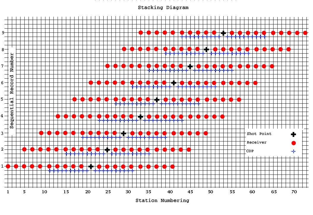
Now, all indexing necessary for sorting will be relative to the Station Number axis at the base of the diagram. The base unit here corresponds to the CDP interval as that is the smallest increment in the acquisition. In magnitude this would be a 12.5 meter station spacing. Group Station indexing starts from 1 and increments by 2 so that it is always odd and follow the sequence 1,3,5,7,9 etc. The first shot in this example is at a Shot Station Index of 21. Each successive Shot Station Index increments by 4 so that Shot Station Index numbers for this example are also always odd and follow the sequence 21,25,29,33,37 etc. The first CDP Station Index on the line is 11, but since the CDP index is the base increment for this diagram, the CDP Station Index increments by 1 and follows the sequence 11,12,13,14,15 etc.
You can see that full fold in this little example is six. To understand this, consider that for the first sequential shot, the bottom shot in the diagram, the last CDP Station Index is 31. By the time the sixth sequential shot is fired the very first CDP Index in that record is also 31. No subsequent shots result in a live CDP located at that position.
Each common shot record contains 20 traces. The near offset is always 25 meters, the far offset is always 250 meters in both directions. The trace spacing within the record is 25 meters.
A common receiver record contains a maximum of 10 live traces at full fold. To understand this consider the last receiver of the first sequential shot [Receiver Station Index 41]. There will be 9 successive shots possible before the spread advances past the point where this receiver will be live. After that, no further energy will be recorded at this position. The trace spacing of common receiver records is 50 meters. This corresponds to the field shot interval of 50 meters used in this example. The near offset will alternate between 25 and 50 meters depending on which Receiver Station Index is considered. Likewise the far offset will alternate between 225 and 250 meters.
A common depth point record will contain a maximum of 6 live traces as discussed above. The trace spacing is also 50 meters. The near offset alternates between 25 and 50 meters, again with a corresponding far offset of 225 to 250 meters.
By installing such a station indexing scheme into the headers of the recorded dataset we can easily form common shot, receiver, offset or cdp records at any point in the processing.
With the above in mind, lets take a close look at our Line_001 for in real life it is seldom the case that everything proceeds in such an ordered fashion. In marine surveys you have currents that push the source and receivers away from their ideal locations. On land you may not always be able to place a group or shot exactly where you would like so one often has to contend with skids of the shot and possible offsets of the groups away from the basic survey design.
In our case, the survey files are built with the shot and receiver numbering already being assigned to an underlying station numbering scheme. For instance the first field record [231] contains a field shot point number of 701. The live field group numbering extends from 561 to 842 the midpoint of which is somewhere between field group number 701 and 702. The contractor indexing scheme has placed this shot at station 701. The real world coordinates of the associated shot and group we see that they are not exactly the same [ shot - (688081.8, 3838302.1), group - (688056.8, 3838384.4) ]. Actually field group number 702 [688081.6, 3838388.0] is actually closer to this particular shot. As we look further into the dataset the station indexing assigned is closer than this most of the time [i.e. shot station 863 (692060.4, 3839098.6), receiver station 863 - (692068.2, 3838952.3)]. A binning scheme, based on the inline projection of the shot was used to assign these shot station values.
While it is nice that some type of station indexing is native to the field shot and group numbering of this dataset it is unfortunate that the group indexing increments by unity. This doesn't leave room in the indexing for CDP indexes which will fall in between the groups and require a floating point scheme. There are lots of schemes to get around this [as our header entries are all integer in this regard]. The easiest for us would be to assign a station indexing scheme that starts at 1 with the first receiver group on the line. Subsequent Group Station Indexes would increment by 2 so that all Group Station Indexes on the line are odd and follow the sequence 1,3,5,7,9 etc. This would put Field Group 701 at a Group Station Index of 281. The first Field Shot location is located here as well. The initial Shot Station Index would then also be 281. The Shot Station Indexing would increment by 4 to account for the nominal field shot point interval of 50 meters. The Shot Station Indexing then would always be odd and follow the sequence 281,285,289,293 etc. The very first CDP Station Index on the line would then be 141 and since the CDP interval is the smallest increment on the line all CDP Station Indexes would increment by one and follow the sequence 141,142,143,144 etc.
There are lots of ways in FreeUSP to load the survey information into the associated field data. We have programs such as laip (land acquisition indexing program), maip (marine acquisition indexing program to perform these tasks. They work very well if you simply want to install an indexing scheme and don't really care about the actual surface coordinates associated with your data. In our present case we would like to honour the source and receiver X,Y data available to us. The contractor has also supplied a static correction in milliseconds and a surface elevation in meters for both shot and receiver locations which we would also like to retain. Programs like laip or maip require that you reformat the information into a form expected by those codes. For surveys designed and acquired by Amoco in the old days, the survey data arrived in a compatible format. For 3rd party data, such as this, that unfortunately is not the case. So we can either do a LOT of typing, or in the usual FreeUSP spirit we can write a quick routine to do all the hard stuff for us. Guess which way I went?
The above is a new FreeUSP routine which will read our field seismic data in USP format as well as our survey data in the formats supplied and install all indexing for you. The field coordinates for source and receiver are stored and well as the static and elevation information. The field record numbering as well as field shot and group indexing are retained. The source-receiver distance is calculated for each trace and installed. Sequential record and trace numbering is also installed.
Simply download the tarball to your ${FreeUSP} directory and extract the files. Along with the source code are a man page and an XIKP pattern file [more about that later]. Once you have extracted the files you can change directory to ${DEPTROOT}/usp/src/cmd/survey and issue the command gmake followed by gmake install . At that point do a rehash and if you now do a which survey you should see something like /FreeUSP/dist/bin/survey. You can see command line help by issuing the command survey -h and more detailed help is available using uman survey.
To run the program on our data issue the following command:
survey -N Line_001.usp -ns 3 -soff 281 \
       -S Line_001.SPS -R Line_001.RPS -X Line_001.XPS \
       -O Line_001.usp_survey
The -ns 3 will result in dropping the auxillary traces from the flow. The following trace header indexing will be installed:
Trace Header   Contents
------------ -------------

InStUn       Shot Static to reference datum in milliseconds
RcStUn       Group Static to reference datum in milliseconds
SrPtXC       Source Point X coordinate
SrPtYC       Source Point Y coordinate
RcPtXC       Receiver Point X coordinate
RcPtYC       Receiver Point Y coordinate
SrRcMX       X distance from source to receiver
SrRcMY       Y distance from source to receiver
RecNum       Sequential Record Number
TrcNum       Sequential Trace Number
SrcPnt       Shot Station Index
SrcLoc       Shot Station Index x10
PrRcNm       Field Record Number
PrTrNm       Field Trace Number
SrPtEl       Source Point Elevation above reference datum
RecInd       Group Station Index
DstSgn       Signed Trace Distance [negative means Group is behind Source]
GrpElv       Group Elevation above reference datum
LinInd       Field Group Number
DphInd       CDP Station Index
SoPtNm       Field Shot Point Number
Now we can get serious in examining this dataset indexing in detail. To get a plot of the Field Shot and Group locations I can issue the commands:
   getval -N Line_001.usp_survey -ne 1 -T SrPtXC -T SrPtYC -O FieldShotCoords
   getval -N Line_001.usp_survey -T RcPtXC -T RcPtYC -O FieldGroupCoords
   usp xgraph -nl -P -bg white -fg black -t 'Survey Coordinates' FieldGroupCoords FieldShotCoords
We can immediately see two things of interest.
Firstly the Field Group locations are layed out in two straight line segments with a change in azimuth between them. The break occurs at the Field Group Number 1055. The first segment [561 - 1055] trends along an azimuth of 81.7 degrees. The second straight line segment [1056 - 1342] trends along 76.4 degrees, a 5.3 degree difference.
Secondly, the Field Shot locations wander back and forth across the axial position of the receiver line and the projection of the shot location onto the line is sometimes coincident with a receiver group and oftentimes nearly equidistant between two groups.
These occurrences are not taken into account by a blind application of some type of station indexing scheme for sorting purposes. We can go ahead and play with the data with such an indexing scheme installed but we must be aware that the spatial relationship of the traces in any of the sorts, including a CDP stack of the data will have some small error in position associated with the image. In FreeUSP there are again many ways to compensate for such skidding of the shots and kinks in the receiver line. In the 2D world that involves supplying an inline skid and angular deviation for every single shot that departs from the scheme. In our case that is pretty much every single shot :-(. It would be much better to jump directly to our 3D sorting schemes that base the sorts and associated binning solely on the source and receiver geographic coordinates. Since this is a tutorial I will show you how to do both. However, before departing from the 2D indexing scheme, let us use what we have installed to get a little more information about the acquisition.
I would like to create a stacking diagram of the acquisition to see just how deviated things become as we move along the line. I could also use this display to spot any problems with the geometry should they exist. A quick way to create such a display is to take advantage of the fact that our line is very nearly following a west to east trajectory. If I add an offset to the Y coordinates of source and receiver in each successive record, then plot the coordinates I will have created such a display. To do that in FreeUSP is pretty easy. First I need to build a quick ufh [Utility From Hell] script to manipulate the headers.
The ufh routine is one of the most powerful utilities we have in FreeUSP. It allows you to recover from just about any problem by operating on the USP trace structure directly. Some people find it intimidating but really you shouldn't. A few minutes of your time spent to go over the ufh tutorial and you will be up and running. There is an archive of ufh scripts on the FreeUSP website to get you started if you are interested. To apply this script to the data and create the desired stacking diagram I can issue the following set of commands:
ufh stacking_ufh < Line_001.usp_survey > Line_001.usp_survey_ufh
getval -N Line_001.usp_survey_ufh -T RcPtXC -T RcPtYC -O stacking_diag_REC
getval -N Line_001.usp_survey_ufh -ne 1 -T SrPtXC -T SrPtYC -O stacking_diag_Shot
usp xgraph -nl -P -bg white -fg black -t 'Line_001 Stacking Diagram' stacking_diag_REC stacking_diag_Shot
There is a lot of data in that plot so to get a better idea how things are progressing as far as the relative shot position is concerned you can zoom in on any section of the xgraph display by drawing a box with your left mouse button held down and letting go. You can resize the resulting display and get better fidelity as a result.
With indexing installed we can now do a quick brute stack of the data to see how things are looking. For the first go-around, seeing has how this is only to QC the indexing, I won't even bother with an onset mute, normal moveout or any other process that one would usually apply prior to stack. I will simply sort to the common depth point domain and stack the data. We can then take a look at the resulting stack and fold plots and make sure nothing looks to amiss.
To do all of this, issue the following commands:
presort -N Line_001.usp_survey -O sort_table
sisort -N Line_001.usp_survey  -n sort_table -D |\
pstack -O Line_001.usp_survey_STACK -F Line_001.usp_survey_FOLD
The presort step creates a sort table containing all information required to do any kind of sort on the data. You can read the man page on the routine for more information. About all you need to know now is that if you issue the command:
head sort_table
you should see:
           -1
     70782
       782       141       251       282      1282        71      5738        72
     1      4
     1   2810    141      1      1      1      1      1      1      -3524    164      1      -3524
     3   2810    142      1      2      1      2      1      2      -3524    165      1      -3524
     5   2810    143      2      1      1      3      1      3      -3524    166      1      -3524
     5   2810    144      1      3      1      4      1      4      -3524    167      1      -3524
     7   2810    145      2      2      1      5      2      1      -3524    170      1      -3524
     7   2810    145      1      4      1      6      1      5      -3524    171      1      -3524
The negative one on the first line basically tells us that all is well.The sisort step reads the sort table generated by presort and the sort type requested, in this case -D specifies common depth point, and feeds up the data in CDP sorted order. The data is then piped into pstack which outputs both a stacked and sample-wise fold dataset. You can plot these in xsd. You can also interleave these by loading them both to the global window and detect interleave. The stacked dataset is normalized for the number of live samples at every sample location. The fold dataset lets you know what that distribution of sample-wise fold looked like.
Last time in we looked at indexing this line using a 2D roll-along scheme projected onto a station index metric. Today let us see what this acquisition looks like if we utilize one of FreeUSP's 3D binning routines to set it up. The programs we will use are sr3d1 to build the sort table and sr3d2 to do the binning.
Before we can run either we need to set up the project corners for the binning. I whipped up a quick ufh script to query the incoming dataset for minimum and maximum source, receiver and midpoint X,Y coordinates.
Running this on our dataset yields:
ufh xylimits_ufh < Line_001.usp_survey

 Source Coordinates
 Minimum Source X Coordinate = 688082
 Maximum Source X Coordinate = 700400
 Minimum Source Y Coordinate = 3.8383e+06
 Maximum Source Y Coordinate = 3.84054e+06

 Receiver Coordinates
 Minimum Receiver X Coordinate = 684590
 Maximum Receiver X Coordinate = 703808
 Minimum Receiver Y Coordinate = 3.83787e+06
 Maximum Receiver Y Coordinate = 3.84128e+06

 Mid-Point Coordinates
 Minimum Mid-Point X Coordinate = 686336
 Maximum Mid-Point X Coordinate = 702104
 Minimum Mid-Point Y Coordinate = 3.83808e+06
 Maximum Mid-Point Y Coordinate = 3.84088e+06

 Total Live Traces = 70782
The following corner coordinates can be used for source, receiver and cdp binning:
(x1,y1)  -->    (684694, 3837309)
(x2,y2)  -->    (705621, 3840999)
(x3,y3)  -->    (705517, 3841590)
(x4,y4)  -->    (684590, 3837900)
They provide enough of a crossline offset to enable us to collect up all bin centers along the line.
Using sr3d1 to create a 3D sort table for this line allows us to experiment with coverage. Lets use a 12.5 meter inline crossline bin dimension so that we can see how the deviation of the source position from the receiver line affects the subsurface coverage. Along with the sort table we will also request a fold plot and azimuthal range and offset range datasets as output:
sr3d1 -N Line_001.usp_survey \
      -x1      684694 -y1     3837309 \
      -x2      705621 -y2     3840999 \
      -x3      705517 -y3     3841590 \
      -x4      684590 -y4     3837900 \
      -dmin -10000 -dmax 10000 -ddel 200 -dy 12.5 -dx 12.5 \
      -F FOLD -S Offset -A Azimuth -O sr3d1_sort_table
Examining the sr3d1 printout file we see that the above parameters afford us 1700 inline and 48 crossline bins and that 70782 live traces were found to be within the corner coordinates used. The maximum fold reached was 20. The minimum source - receiver offset was 12.04 meters. The maximum offset reached 3524.8 meters.
The FOLD dataset generated is in USP format and can be plotted in xsd. To duplicate the plot use a horizontal zoom of 4, min-max scaling and the Fold_Color colourmap. Corner 1 (x1,y1) is associated with (trace 1, sample 1) and is located in the top left corner of the plot. Corner 2 (x2,y2) is associated with (trace 1, sample 1700) and is located in the bottom left. Continuing in a counter clockwise rotation are corners 3 and 4. You can see that the subsurface fold extends from sequential crossline bin 13 through 45 and from sequential inline bin 142 to 1421. On average, the subsurface coverage of the acquisition is about 10 bins wide. We can readily see that the excursions made by the source location across the line results in a spread in the calculated midpoint of some 125 meters.
The Azimuth dataset is in ASCII format and can be plotted using:
usp xgraph -P -bg white -fg black -t 'Source - Receiver Azimuth' -y 'Histogram Frequency' -x 'Angle in Degrees' Azimuth
and shows predominent source - receiver angles of near 75 and 255 degrees which is consistent with split spread shooting along the azimuth range of the receiver line. The spread of angles near these maxima is indicative of the offset of the source location away from the line.
The Offset dataset is also in ASCII format and can be plotted using:
usp xgraph -P -bg white -fg black -t 'Source - Receiver Offset' -y 'Histogram Frequency' -x 'Offset in Meters' Offset
and shows a fairly even distribution of offsets between 12 and 3524 meters. There is a little hump in the distribution toward the near offset.
This is all well and good but processing this line as a 3D volume won't help us in this 2D tutorial. So rather than going on to create an arbitrary traverse down the maximum fold we will simply make the crossline bin dimension large enough to encompass all the data:
sr3d1 -N Line_001.usp_survey -O sr3d1_sort_table \
-x1      684694 -y1     3837309 \
-x2      705621 -y2     3840999 \
-x3      705517 -y3     3841590 \
-x4      684590 -y4     3837900 \
-F FOLD -S Offset -A Azimuth \
-dmin 0 -dmax 4000 -ddel 200 -dy 12.5 -dx 600.
A cursory stack of the line using the sr3d2 routine can now be performed. It does require two passes. The first reads in both the input seismic data and the sr3d1 sort table and creates what we will call an sr3d2 volume. This is the input data arranged on disk in the order required to feed up sequential binned gathers. This makes all subsequent call to sr3d2 go much faster, assuming of course that you are feeding up data sequentially which we usually are. [Next time in I will add a section showing the use of the 3D routines dbvec and edit3d which don't require the extra volume and are a little more flexible in how the data may be ordered on retrieval.] The second pass, and all subsequent passes, simply feeds up the gathers as requested. The FOLD output indicates 1700 inline bins with only 1 crossline bin as expected. The Offset and Azimuth information is unchanged but the maximum fold reached is now 71.
The following command line entries will create the sr3d2 volume and then go on to form a quick stack of the data, again with no attempt at an onset mute or even normal moveout:
sr3d2 -N Line_001.usp_survey -P sr3d1_sort_table  -D sr3d2_volume -stop
sr3d2 -P sr3d1_sort_table  -D sr3d2_volume -go |\
pstack -O sr3d2_STACK -F sr3d2_FOLD
The resulting stack and stack/FOLD interleave show a similar [though subtly different] picture to that due to the 2D indexing above.
That is it for tonight, I have a rough week this coming week and might not get back to this until near week's end. When I do I will show you one more way of binning this data using our vector database and 3D editing capability. That approach allows for quick sorting, and stacking, in either common shot, receiver or depth point domains. You can also call up macro-bins of data for velocity [or other] analyses as you wish.
For today's lesson you will need to download, compile and install an upgrade to two FreeUSP codes [dbvec and edit3d].
Copy these files to ${FreeUSP} on your machine and untar them. Change directory to ${DEPTROOT}/usp/3d/src/cmd/dbvec and do a gmake clean, gmake and gmake install. Do the same for edit3d. I discovered to my horror, while building this section of the tutorial, that these codes were broken on LINUX. If your copy of FreeUSP includes a patch or release date later than April 12, 2005 you most likely already have the fix installed and do not need to perform this step. You'll find out quickly enough for if you have the old codes installed they will crash when you attempt to run today's exersize.
So far we have indexed the data using both a projection to 2D and a common mid point 3D binning system. FreeUSP offers another option utilizing the vector database routines, dbvec and edit3d. dbvec serves a purpose similar to presort in the 2D scheme or sr3d1 in the basic 3D scheme in that it creates a table for use in sorting the input dataset. edit3d serves the purpose of sisort [2D] or sr3d2 [3D] in that it reads both the data and the vector database in order to supply gathers sorted according to wishes of the processor. Being a 3D process, dbvec requires the common mid point grid corners as previously supplied to sr3d1.
Unlike the 2D routines, this pair of programs works from the actual (x,y) source and receiver coordinates of the data to populate common mid point bins. Unlike sr3d1 / sr3d2, no intermediary disk sort is required and in addition to common mid point gathers, you may also sort to any one of common shot, common receiver or macro-binned mid point as you so desire. For a given 3D grid there is no difference between a common mid point dataset served up by sr3d2 and that coming out of edit3d.
We will use the full power of dbvec and edit3d when we go on to create a 3D processing tutorial. Here we will simply introduce the programs and demonstrate their functionality as applied to this crooked line 2D example.
So, the first step is to create the vector database. We are going to skip generating a finely binned system in the crossline direction and proceed directly to the use of wide bins to compensate for the crooked line nature of the input dataset:
dbvec -N Line_001.usp_survey \
      -O dbvec_database \
      -hwshot SoPtNm -hwgroup RecInd \
      -dx 600. -dy 12.5 \
      -x1 684694 -y1 3837309 \
      -x2 705621 -y2 3840999 \
      -x3 705517 -y3 3841590 \
      -x4 684590 -y4 3837900 \
      -dmin 0 -dmax 5000 -ddel 25
We can now generate common mid point gathers and a brute stack of the input:
edit3d -N Line_001.usp_survey -DB dbvec_database \
       -dis 141 -die 1423 -ddi 1 -U |\
pstack -O edit3d_CMP_STACK -F edit3d_CDP_FOLD
The resulting stack is identical to that produced using sr3d2. We don't have to stop here as we now have the power to quickly sort to common receiver gathers and create a common receiver stack of the input:
edit3d -N Line_001.usp_survey -DB dbvec_database \
       -rcst1 1 -rcst2 1563 -rcinc 2 -sopt -U |\
pstack -O edit3d_RECEIVER_STACK -F edit3d_RECEIVER_FOLD
The resulting stack and fold overlay show the fold building up and dropping off at each end of the acquisition.Common shot gathers along with a subsequent stack are also easily served up. For this example one may rightfully argue that to get this sort we need only grab the input data as is. True, but if the input data was not already in a shot sorted order this is the statement that would be required to form such an output:
edit3d -N Line_001.usp_survey -DB dbvec_database \
       -shst1 701 -shst2 1201 -rcinc 2 -sopt -U |\
pstack -O edit3d_SHOT_STACK -F edit3d_SHOT_FOLD
Here the resulting stack and fold information reflect the fact that there are a constant number of receivers turned of for each shot. The fold is constant at 282 for all samples which is the number of traces per record on all shots in this acquisition. Once we apply normal moveout and install a mute that will change as a function of time.
Initial Signal Analysis and Quality Control
For today's lesson you will need to install an upgraded binary for bdmute. While doing the processing I found that the FreeUSP bdmute code directory contained an old cmdln.F routine. I don't know how that happened but here is a tar file update for bdmute that corrects this problem with the FreeUSP distribution:
To install this code, download the above to ${FreeUSP}, untar the file, change directory to ${FreeUSP}/trcgp/usp/src/cmd/bdmute, run gmake clean, gmake, gmake install followed by a rehash.
For the remainder of this tutorial we will make use of the 2D indexed data. We'll save working with the 3D programs for a future 3D tutorial.
visual QC of field shot data
Our first order of business is to become very familiar with the signal and noise characteristics of this acquisition. Since this is such a small dataset we have the luxury of examining every shot record visually. Plot the entire dataset in sets of N records [ N can be anything you are comfortable with, I used N = 50] in xsd. Use a maximum scalar of 40, an exponent of 1, set sample delta and origin as 2 and -2 respectively, plot every trace and every record using vertical and horizontal zooms of 1.0 and the gray4 colourmap. You can alternate with the gray colourmap as you like but be sure to use the gray4 colourmap initially to highlight outlier amplitudes.
Sequential shot record 198 is a typical example. It corresponds to the field shot record 1095 [ shot station index of 1069]. Prior to the first breaks low amplitude noise, rumbling around in the subsurface prior to the shot, is recorded by the array. We will mute this energy by designing a first break mute to apply to the data. The first breaks correspond to the direct compressional surface wave energy refracted along the first couple of subsurface layer interfaces. These waveforms arrive at the geophone with a much higher amplitude that reflections from depth. The two slope breaks along this set of arrivals correspond to a refraction arrivals from the first two distinct layers in the near surface. We can measure the velocity at which these arrivals traverse the recording array and derive the layer velocity associated with these zones. More on that later. The extremely high amplitude arrivals constrained to a tight cone in the very near offsets are due to ground roll generated by the vibrator source. These arrivals are heavily aliased due to their very slow propagation velocity. Our 25 meter geophone spacing is insufficient to record these arrivals unaliased. The boundary of the high amplitude zone defines a velocity near 300 or so meters/sec which of course is very close to the speed of sound in air. Trace 69 contains some type of electrical noise from that group. This is typical of a receiver whose wiring has been damaged, or has a bad ground.
To fully understand the genesis and physics of the arrivals observed in this record you should review Notes on Geophysics as Applied to Land Seismic Acquisition by Andy Pap. Pay particular attention to the section entitled The Seismic Noise
As you examine the data, make a table of any data problems that you see as you go along. Record the sequential record and trace along with the observed signal problem.
datum statics, deterministic scaling and first break mute
Supplied with the survey data are shot and receiver elevations as departure in meters from a regional datum. These quantities are stored in the trace header mnemonics SrPtEl and GrpElv respectively. The replacement velocity used to reduce the recording surface to the regional datum is specified as 1900 m/sec in the Line_001.TXT file which accompanied the basic data.
We apply shot and receiver datum statics using:
word_swap -N Line_001.usp_survey -hw1 SrPtEl -hw2 Horz01 -amp 0.526316 |\
rest -SW Horz01 -F -u -1.0 |\
word_swap -hw1 GrpElv -hw2 Horz02 -amp 0.526316 |\
rest -SW Horz02 -F -u -1.0 |\
ttothen -exp 2 -O Line_001.usp_survey_datum_ttothen
where the quantity 0.526316 comes from (1000.0 / 1900.0) to convert the shot and receiver deviations from the regional datum in meters to a corresponding time static measured in milliseconds. Since all the measurements are positive we will subtract the static to reduce the source and receiver positions to the regional datum.
word_swap reads the appropriate distance in meters from the trace header entry specified by -hw1[], multiplies by the conversion factor -amp[] and stores the resulting floating point static, in milliseconds, in the trace header mnemonic indicated by -hw2[]. The rest routine performs a phase shift in Fourier space to apply the source and receiver datum statics.
ttothen applies a deterministic tn scaling to each trace. This scaling compensates, to a first order, for the energy loss due to spherical divergence as the wavefront propagates into the earth and back. Being deterministic, this scalar can, and will be removed, at a later stage in the processing. Its application here is simply to ease the task of upcoming signal analysis on this data.
We are not interested in seismic arrivals prior to those generated by the source. Such background noise, recorded prior to the first break from the actual shot, need to be muted from consideration.
There are many ways in FreeUSP to parameterize a first break mute. mute allows the user to define the onset mute as a function of velocity across the receiver array. bdmute allows one to actually pick the mute trajectory interactively in xsd and pass the mute parameters to the program in the form of an xsd pick file or alternately an xsd header value at pick location file. Since our first breaks represent more that a single velocity we will pick a mute in xsd and apply it using bdmute.
I first plotted every tenth sequential shot record from record 1 through 251. I then cleared the pick register in xsd by detecting New Segments from the xsd File pull down menu. This makes sure that no previous picks are hiding in the register. When we are finished picking and export the resulting picks, all picks in the register will be output. If you have been messing with picks on previous images, those picks will still be in the register and will end up in your mute control pickfile. If this should happen, bad things are sure to follow.
Picking is always on in xsd. To initiate a pick segment you simply place the cursor at a desired location and click your left mouse button. To back up on a pick segment, use your middle mouse button. To end the segment, click on your right mouse button. For kicks I first choose a pick colour by clicking on Pick Color on the Color pull down menu . I detect red from the resulting pick colour menu and then cancel. Now all my picks will turn up as red in the frame.
Starting from the left side of the first record I pick a first break mute by repeatedly clicking my left mouse button along the event of interest. Once I have reached trace 282 I click on the right mouse button to end the segment. If I make a mistake or wish to backup while picking I simply click on my middle mouse button. Once the pick segment is ended with a right mouse click I can still modify it by going to the Move Picks or Delete Picks entries on the Picks pull down menu in the window.
Once I am happy with the pick I can copy that pick to all other records of the display using the Copy Segment From/To entry in the Segment pull down menu . In this case I copy the picks from record 1 to records 11 through 251 every 10. As soon as I hit return I see the first break picks from record 1 appear on all records of the display.
I can now review each record, moving, adding or deleting picks as required to fully parameterize the mute.
I save the picks into an xsd pick file by detecting Save Segments on the File pull down menu of the window [ note that the file pull down menu contains different entries if you detect it in a data window as opposed to detecting it in the xsd mother widget]. I can also choose to save the pick information as a header value at pick location file by clicking on the Save Trc Header entry of the File pull down menu. Once I enter a file name I will be presented with a menu allowing me to choose any number of trace header values to include with the pick information. For the case of a mute I am interested in adding the signed trace distance DstSgn to the output. It is not necessary to output both types of pick files as the first output is sufficient for what we are attempting. If you do need to parameterize for an offset mute, be sure to always output a regular xsd pick file in addition to your header value at pick locations file. The header value at pick location file cannot be reloaded to xsd to display picks at some future date. Only the regular xsd pick file can serve that role.
To apply the first break mute utilizing the standard xsd pick file, run:
bdmute -N Line_001.usp_survey_datum_ttothen \
       -P mute_picks -M on \
       -O Line_001.usp_survey_datum_ttothen_bdmute
To apply the first break mute utilizing the xsd header value at pick location file, run:
bdmute -N Line_001.usp_survey_datum_ttothen \
       -P mute_header_picks -M diston \
       -O Line_001.usp_survey_datum_ttothen_bdmute
You should be good to go at this point. Once applied we are ready to start tearing this data apart in earnest.
time-frequency analysis
The ground roll and any associated air disturbance close to the vibrators is picked up by the near offset phones . This combination is the most destructive noise on the data. It forms a cone shape region below the source known in the trade as the "Cone of Despair". Many techniques have been developed over the years to increase the signal to noise ratio in this zone. Some of these techniques can be applied during acquisition, others during processing.
The first I will pull out of our processing hat is the stft routine which allows us to perform a time-frequency decomposition of the input data.
For today's lesson you will want to install an upgraded binary for smute. I added -threshold[] capability for use with our stft routine to allow for time-frequency thresholding of the data.
To install this code, download the above to your ${FreeUSP} directory, untar the file, change directory to ${FreeUSP}/trcgp/usp/src/cmd/smute and run gmake clean, gmake, gmake install followed by a rehash.
We left off last time looking at the "Cone of Despair" and were about to decompose the data in time-frequency. Let's work with our sequential shot record 198 for illustration. I have windowed the record to 2950 ms to remove the hard edge that appeared when the source and receiver statics were applied:
editt -N Line_001.usp_survey_datum_ttothen_bdmute -rs 198 -re 198 |\
wind -e 2950 -O rec198
Fire up the FreeUSP specal program using:
specal &The specal gui will appear on your screen. Click on the File pull down menu and detect Select File at which point a file selection gui will pop up. Detect your rec198 dataset by double clicking on it. You will now be presented with a new parameter entry panel. Detect a 2D transform, use all the traces in the gather and set the end time at 2950 ms, as there is no data past that point in the record, then click OK. The 2D Fourier transform of the selected data should now be on the screen. It may look odd for the default colourmap may not be appropriate for your data. If this is the case for you, then detect ChangeColorScale to bring up the Color Editor. Detect Change Limits, set the lower amplitude limit to zero and the upper to about 1000 then click OK. You may now use the colour palette and action when palette color is picked options to place colors and interpolation points into the color axis on the left hand side of the gui. Once you have your choices completed click on the Interpolate Colors button then Apply. The resulting changes to the colourmap will then be transfered to the displayed spectra.
The specta clearly shows the upper and lower frequency limits of the vibroseis sweep [8 - 95 Hz]. Carrying forth with 2 millisecond sampled data [Nyquist frequency 250 Hz] is clearly not required. We will resample to a 4 ms sample rate [Nyquist frquency of 125 Hz]. Since there are no frequencies above 95 Hz in this data we do not strictly need to first apply an anti-alias filter prior to resampling. However, since this is a tutorial, we will not make any such assumptions and go ahead with the design of an anti-alias filter, to be applied prior to resampling, that will attenuate all amplitudes above 125 Hz to below 60 db down.
We need to examine both the time domain impulse response and frequency domain equivalent, the transfer function, of our anti-alias filter to ascertain that the filter will perform as required. To obtain the impulse response from our filter we can convolve the filter, in the time domain, with a spike. To create such a spike use:
spike -O spike -L 2950 -t0 1476 -ntr 1 -gi 10 -si 2To view the resulting time series and make sure that the spike is truly a spike use:
sis_xy -N spike | morego on down to the entries near 1476 milliseconds and make sure the spike has been assigned to a single sample and not split between two adjacent samples. In our case you will find:
     1470.00000      0.00000000E+00
     1472.00000      0.00000000E+00
     1474.00000      0.00000000E+00
     1476.00000      0.10000000E+01
     1478.00000      0.00000000E+00
     1480.00000      0.00000000E+00
     1482.00000      0.00000000E+00
You can also plot the spike trace using:
sis_xy -N spike | usp xgraph -bg white -fg black -t 'spike trace'To view the transfer function we transform the observed time domain impulse response to the frequency domain. This is easily done using specal. Note that the frequency domain equivalent of a spike in time is a level in frequency. This should not be too surprising as the single spike amplitude is being sampled at all frequency decompositions.
You can play filter design games to your heart's content now. Simply choose your favourite filter design, apply it to the spike dataset, plot the resulting impulse response in time and load the impulse response dataset to specal to view the frequency domain transfer function. Here is one filter that will do the trick:
filt -N spike -O spike_filt -fl 6 -fh 85 -nor 6 -MNote the -M on the filt command line. This entry causes the program to NOT restore the mute to the input dataset. This is required when filtering a spike otherwise the program will restore both the on and off mute [based on presence of hard zeroes on the input trace] which will wipe out the sidelobes of your impluse response it not turned off. If you notice that the spike is still a spike after filtering, but that the spike has a lower amplitude, check to make sure you have the -M on the filt command line.
Again, to view the impulse response use:
sis_xy -N spike_filt |usp xgraph -bg white -fg black -t' Butterworth 6 - 85 Hz, order 6'and to view the transfer function, load the filtered spike to specal and plot the 1D amplitude spectrum [log scale]. See if you can design one for yourself. I have used a Butterworth filter, you can choose to use an Ormsby if you wish [or any other filter you care to experiment with].
Once you have a filter that provides protection against aliasing you may apply it to the real data and do the resampling. In FreeUSP, we can do both at once with program filt since our target sample rate is an integer decimation of the original:
filt -N rec198 -O rec198_4ms -fl 6 -fh 85 -nor 6 -M -d 2If it was not, then you would use filt to apply the filter and gentrp to do the resampling. A scan of the resampled data shows the changes made to the line header:
scan -N rec198_4ms | more

  line header values after default check
  # of bytes in line header=        2658
  # of bytes in output line header=        2678
  # of samples/trace =           738
  sample interval    =             4
  s.i. multiplier    =    1.0000000E-03
So we now have 738 samples per trace and a sample interval of 4 milliseconds.
We are now ready to take a look at this data in time-frequency space. To perform that transform use stft:
stft -N rec198_4ms -O rec198_4ms_stftThe stft algorithm employs a 32 sample running window short time Fourier decomposition of the input data. Using the default parameters, each input record is decomposed into [ 32 / 2 + 1] or 17 frequency sub-bands between DC and Nyquist. The first half of each output trace contains the spectral amplitude coefficients, the last half the phase. Unlike a stationary 2D Fourier transform of the entire record, the time-frequency decomposition allows you to localize the temporal and spatial distribution of energy within each frequency band.
Plot the spectral amplitude portion of all 17 subbands in xsd using a maximum scalar of 2.0. Install the Fft2daColor colourmap. You can see quite clearly that this decomposition is quite different from the stationary transform seen previously using specal.
The high amplitude data in the "Cone of Despair" is spatially aliased and turns up in the stationary transform as a band of energy, seemingly independent of wave number, extending from 12 to 30 Hz with a peak spectral amplitude near 16 or 17 Hz. The time-frequency decomposition shows this same signature. In contrast however, it does allow one to isolate the energy in time and space, which is impossible using the 2D stationary Fourier decomposition. We can now experiment with amplitude attenuation within the cone, perform the inverse transform and watch what happens. To perform the subband dependent thresholding we will use the upgraded smute routine that I had you download and install at the start of today's session.
Here is a thresholding scheme that gets us started:
stft_splitr_jobThis script, which applies a selected threshold to only the portion of each subband over which the noise is dominant. It requires the following file lists:
stft_fileout
stft_fileback
To run this script on our data, use:
stft_splitr_job rec198_4msThe file rec198_4ms_denoise will be produced which you can plot in xsd. You will want to plot this record using a fixed scalar equal to that used to display the original data. You will also want to create a difference record so you can see exactly what you filtered out:
vstak -N1 rec198_4ms -N2 rec198_4ms_denoise -amp -1 -O rec198_4ms_diffYou can plot this record in xsd as well, again using the same fixed scalar so that all three records are plotted with the same amplitude reference. If you don't do this, xsd will scale each record individually and you will not see a relative view of what has transpired.
Wow, it has sure been a long hiatus since I last found time to work on this project. Sorry about that. As you might imagine, with all that has been going on with BP in the Gulf of Mexico this summer, things have been fairly hectic at work. So, where were we!!
I see we had made an attempt at knocking down the energy in the cone of dispair. We had also resampled the data to a 4 millisecond sample interval. Before going on to an initial velocity analysis, in a tutorial spirit let us look at an alternate method for applying the stft time - frequency filter using the USP iconic processing engine XIKP. XIKP is a graphical flow builder, which some people prefer over script construction for complicated flows. It allows for easy construction and execution of topologically complex processing flows, flows so complicated that they simply cannot be reproduced in script mode in anywhere near the same time frame. I am not going to do a full description of the tool, but merely show how to do the immediate processing. There is an excellent XIKP tutorial on the FreeUSP website for those who wish to know more.
On the command line, enter:
XIKP &and hit return. You will be presented with the XIKP graphical front end. If not, then you may not have all the support for XIKP set up on your system. Look through the installation guide in the XIKP tutorial and perform the tasks required to activate the ikp daemon. If this is beyond you, then just follow along; later on you can get someone with some system savy to set you up.
We need to create a filter for stft as a first step. To do this go to the create pull down menu and detect filter. Now move your cursor into the graphics area to the right and you will see an angle iron denoting the position of the top left corner of the filter icon. Move this to a position of your choice and hit your left mouse button. A graphical filter should now reside in the graphics area. The solid arrows pointing in on the left and out on the right are stdin and stdout. The dotted arrow pointing out at the bottom is stderr. If you click on the icon with your left mouse button you will get up a filter menu into which you may enter any valid Unix command; in this case stft. Hit OK on that menu after entering stft and you will see the graphical display of the filter now indicates the command that is being executed. Now go to the library list, scroll down to trace editting and double click. You will see a list of modules appear in the window below. Scroll down in that list until you see splitr1to17 and double click on that entry. Drop the splitr icon into the graphics area. We can connect stdout from stft to stdin of splitr by placing your cursor in the goal post area of stdout on the stft icon and clicking your middle mouse button. You will see a couple of arrows appear, pointing at the stdout connector, now place your cursor in the stdin goal post area of the splitr icon and click your middle mouse button again. You will see a connector line appear connecting the stdout of stft with the stdin of splitr. It takes a little practice at first to get your cursor in just the right place, but eventually you should get the hang of it. Now scroll in the module list to merge17to1; double click on it and place the merge icon in the graphics window. Create another filter icon and enter the command to do the inverse stft on the command line. Connect the stdout of the merge icon with the stdin of the stft inverse icon. Your forming XIKP net should look like this.
The splitr process, by default, takes incoming records and sprays them sequentially over the 17 output spigots, exactly like a distributor cap. The stft process, as we are using it, creates 17 frequency sub-band records for each input record, so you may now be getting the idea that each spigot of the splitr process is going to correspond to a single frequency sub-band of the stft decomposition.
The merge process, by default, picks up incoming records and composes them into a single output stream on the stdout of the process. The incoming records are picked up back to back in exactly the opposite fashion as they are sprayed out by splitr. This is like an anti-distributor cap. The data flow is then directed into the inverse stft process and time domain data, one record for each 17 input records, will be passed to stdout of that process.
Now comes the interesting part. We can filter each frequency band in a unique fashion, or choose to do nothing at all, very easily. Scroll to the Muting category in the library list, double click, and choose the smute routine from the module list. Place the smute icon in the graphical area and click on it. Fill out the menu items accoring to the associated smute from the script above. Notice that there are two smute entries associated with the first sub-band. So get another smute icon and set its parameters to those of the second smute for that sub-band. Connect the flow for sub-band 1 so that data flows from the splitr through the smutes to the merge. Now repeat this process for sub-bands 2 through 7. Sub-bands 8 through 17 are simply connected directly between the splitr and merge as that data is passing through the process unfiltered. Your net should look something like this. During this construction process you can copy icons already created, which also copies their parameters. This makes life a little easier. You can also move things around to make room for everything. See the XIKP tutorial for help in this area.
Finally we add input and output dataset by simply hitting f on the keyboard, moving our cursor to the stdin goal post area of the stft icon and clicking our left mouse button. You will be presented with a file selection box in which you can browse to your desired input dataset and detect it. Do the same for the stdout connection to the inverse stft process and your net is complete. You can save the whole net by detecting save as from the file pull down menu. As you move your cursor into any element of your net and click your left mouse button. All processes connected to that icon will be highlighted and a save net selection box will pop up. Enter a filename for your net and click ok.
You can execute this net in one of two ways. Firstly you can execute it in interactive mode by clicking on the run entry in the net pull down menu. Move your cursor to any element of the net and click your left mouse button. The net will fire up and assuming no mistakes will run to completion. All stderr messages will end up in the window where you started XIKP. This is fine for testing the net, and for small datasets. For larger datasets you can start the net in batch using:
nohup XIKP -B stft_net >&! stft_net_messages&
In this case the net will fire off in background and all stderr output from the various processes will be directed to the messages file. The beauty of the second approach is that you can submit this job, log off and go home. It does not depend on an active X server to stay running. The initial method suffers from the weakness that should your X environment go south, so will your job.
This has been a bit of a diversion from actual seismic processing, but some may find it interesting. Here is the net I actually ran. You can stuff it in a file and load it to XIKP using:
XIKP -N stft_net &
You can then connect to your input and output files of choice and fire it up.
Before we can get into the next phase of noise suppression, which involves filtering in all three sort domains, shot [CSP], receiver [CRP] and common mid point [CDP], we need to do something to increase leverage between primary reflected events and the massive amount of linear noise associated with this acquisition. Normal moveout provides a method to achieve this, but with the data in its current state it will be very difficult to utilize velocity semblance spectra to derive a set of stacking velocities.
If you would like to see how desperate things are, sort the data to CDP, find a gather where you think you can identify something other than noise and generate a velocity semblance spectra for that record. I have done exactly that using:
sisort -N denoise_4ms_CDP_nmo_CSP_fft2da_poly_back \
       -n sort_table -D \
       -O denoise_4ms_CDP

velspec -N denoise_4ms_CDP \
        -O velspectra -vmin 500 -vmax 5000 -nvel 300 -A
I have then loaded the spectra and gathers into our vxos velocity picker. It is not possible to contemplate using this tool with the data in its current shape. I will leave description of it's use for later. Note that the S/N of the data is so poor that picking a stacking velocity trend is problematic to say the least.
Lets try another approach, that is more amenable to poor S/N data. We can generate a suite of constant velocity stacks over a range of likely velocities and hope to see something in the data that we can key on to generate a rough stacking velocity field. I create the required constant velocity stack dataset using:
#! /bin/sh -f
#
file="denoise_4ms_CDP"

for velocity in `cat vellist`;do

bdnmo -N ${file} -cv ${velocity} -E |\
mute -R |\
pstack |\
utop -R 1 -L 1282 |\
apend -O VelocityAnalysis/cvstack_dataset

echo done ${velocity}

done

echo finished
exit
which uses the file vellist which simply contains a set of velocities, one per line, for the process. For each velocity in the file the data will be moved out, stacked and added to the accumulating dataset. Once the job is finished I can load the entire dataset into xsd as a movie and pick a cursory stacking velocity function set manually. When loading the movie you can utilize xsd server parameter options to have the record number turn up on each frame as the velocity of that frame. To do that simply make the Delta for the record entry correspond to the delta v from your vellist file. The Origin would then be the first velocity in the file less the delta.
Luckily for us, the S/N of the constant velocity stacks is easily adequate to allow us to define a stacking velocity function along the line. The power of stack allows us to clearly see events come to focus at varying velocities, thus allowing us to catalogue those time,velocity entries as a spatial stacking velocity function:
I derived a stacking velocity function at several locations along the line and stored them in a file in the flat file format required by our velocity input routine velin. In this file the first column is time in milliseconds, the second is velocity in the units of the data while the last column is the record number which in our case is the sequential CDP gather number associated with that location in the stack. Once I have this file defined I can generate a velocity volume to fit the stacked data using:
velin -N denoise_4ms_CDP -v cvstack_velocity_function_picks -flat -R -O velusp
Which performs a linear interpolation between functions and between function elements to flush out a velocity volume with a single velocity trace for each gather of the input CDP dataset. This velocity dataset can be plotted in xsd for a quick QC.
To obtain a brute stack of the data making use of the above stacking velocity dataset we first apply normal moveout to the CDP data using:
bdnmo -N denoise_4ms_CDP -v velusp -E -O denoise_4ms_CDP_nmo
We can plot a selection of moved out gathers from the output dataset, pick a typical one and generate a post normal moveout mute for the data. Once the mute is picked in xsd, use the save trc header option to save out the picks along with DstSgn. This allows us to use the distance muting option in bdmute to apply that profile to all gathers of the volume. We can then mute the data and generate a brute stack using:
bdmute -N denoise_4ms_CDP_nmo \
       -P mute_header_picks -M diston -O denoise_4ms_CDP_nmo_bdmute
pstack -N denoise_4ms_CDP_nmo_bdmute -F Stack_FOLD |\
counter -ssam \
        -O denoise_4ms_CDPSTACK
Examination of the brute stack shows that we are starting to see subsurface upgoing energy. If we interleave the stack with the fold stack generated by pstack, we can see how the signal content relates to the number of samples stacked at any given sample location in the data.
So, we are getting somewhere, but we have a long way to go. This stack, though showing something of the subsurface, still suffers from many areas where surface static busts are evident, areas where the linear noise in the data is so strong it is hard to make out the upgoing energy and areas where it looks like our stacking velocities are wholly inappropriate. In addition, there are several zones where the post NMO mute needs to be adjusted. We can do much better than this.
To understand a little more about the coherent noise present on this acquisition it is useful to observe the data in both end point domains, shot and receiver, as well as the midpoint domain, CDP.
Consider the CDP gathers responsible for our brute stack. Notice that with normal moveout applied, even using the cursory stacking velocities derived above, we can see evidence of flat-lying upgoing primary reflections. These reflections are swamped in a sea of spatially aliased noise. Most of this noise is backscattered energy travelling around in the near surface and hence traveling across the receiver array linearly at a pretty low velocity. The CDP trace spacing is about 100 meters which is why the noise looks so spatially aliased in this domain; it is.
If we sort this data back to the receiver domain using:
presort -N denoise_4ms_CDP_nmo_bdmute -O cdp_sisort_table
sisort -N denoise_4ms_CDP_nmo_bdmute -n  cdp_sisort_table -G -O ../Receiver/denoise_4ms_CDP_nmo_CRP
we see that at a trace spacing of about 50 meters some of the backscattered noise is now coherent and unaliased.
If we sort instead, to the shot domain with a trace spacing of about 25 meters using:
sisort -N denoise_4ms_CDP_nmo_bdmute -n cdp_sisort_table -S -O ../Shot/denoise_4ms_CDP_nmo_CSP
we see that a lot more of the backscattered energy is unaliased.
Now that we can start to see some of the signal separation that we were looking for, lets see if we can do something about preferentially attenuating the noise component. We can transform the shot sorted data into F-K space using:
fft2da -N denoise_4ms_CDP_nmo_CSP -O denoise_4ms_CDP_nmo_CSP_fft2da
The more experience among you may start to see the separation of noise and signal in this F-K image. Without a lot of experience in this area it is tough to guess the relationship between event trajectories in T-X and those in F-K. Luckily in the USP arsenal is a routine ich which allows one to pick events in T-X in xsd, convert the picks into a model complete with the trace header structure of the real data, and then transform the model to the F-K domain using:
ich -N denoise_4ms_CDP_nmo_CSP -P ich_picks -S -O denoise_4ms_CDP_nmo_CSP_ich
fft2da -N denoise_4ms_CDP_nmo_CSP_ich -O denoise_4ms_CDP_nmo_CSP_ich_fft2da
This approach allows us to see where the selected primary events lay and more importantly where the picked linear noise is located in F-K space. Armed with this knowledge we can digitize a polygonal filter to pass the signal and eradicate the noise. Once the polygons have been picked for a decent selection of shots we can apply the filters using:
polymute -N denoise_4ms_CDP_nmo_CSP_fft2da -P fft2da_picks_4ms -M out -nxtaper 5 -nztaper 5 |\
fft2da -R -O denoise_4ms_CDP_nmo_CSP_fft2da_poly_back
So, what have we managed to accomplish here. To get an idea, let us look at the shot gathers before and after application of the filter:
Quite a difference. One may argue that we have utilized too severe a filter at this early stage of the processing. That may well be true, but let us not forget that the goal here is to get to a decent statics solution, and then the first iteration of the stacking velocity derivation. To do both of those we need as clean a dataset as we can get. We can always back up later and reduce the attenuation associated with this filter. Although the filter looks a little severe when viewed in the shot domain, what has it done to the data in the other two sort domains? To sort the data to the CDP domain for this display we use:
sisort -N denoise_4ms_CDP_nmo_CSP_fft2da_poly_back -n sort_table -D \
       -O ../CDP/denoise_4ms_CDP_nmo_denoise_CSP_CDP
and here we see:
So, even though the filtered data looked a little wormy in the sort domain in which it was applied, the same is not true of the CDP domain that is being stacked. Here we see a definite improvement in the S/N ratio of this data.
For completeness lets see what we have done to the stack:
A not insignificant improvement, given the crudeness of the filter applied, and only in one domain. As you can see from the difference dataset, there is no indication of any primary event being attenuated in the stack.
And now, what have we done to the Receiver gathers:
sisort -N denoise_4ms_CDP_nmo_CSP_fft2da_poly_back -n sort_table -G \
       -O ../Receiver/denoise_4ms_CDP_nmo_denoise_CSP_CRP
Again, an amazing amount of signal enhancement without the worminess seen in the domain where the filter was applied. We do notice however that there remains quite a bit of residual linear noise that could be attacked in this domain. That noise was not aligned when the data was sorted to the shot domain where the initial filter was designed and applied.
We will perform the same operation here, that is transform the receiver data to F-K space, pick a set of polygonal filters to reject as much noise a we feel is practical, apply those filters in the F-K domain to the receiver sorted data then transform back to T-X and see what we have accomplished.
Here are the processing steps involved:
fft2da -N denoise_4ms_CDP_nmo_CRP |\
polymute -Mout -nxtaper 5 -nztaper 5 -P fft2da_4ms_picks |\
fft2da -R -O denoise_4ms_CDP_nmo_CSP_fft2da_poly_back_CRP

sisort -N denoise_4ms_CDP_nmo_CSP_fft2da_poly_back_CRP -n presort_table_CRP -D \
       -O ../CDP/denoise_4ms_CDP_nmo_denoise_CSP_denoise_CRP
pstack -N denoise_4ms_CDP_nmo_denoise_CSP_denoise_CRP -O denoise_4ms_CDP_nmo_denoise_CSP_denoise_CRPSTACK

sisort -N denoise_4ms_CDP_nmo_CSP_fft2da_poly_back_CRP -n presort_table_CRP -S \
       -O ../Shot/denoise_4ms_CDP_nmo_CSP_denoise_CRP_denoise
Here are the results:
[before] [after] [difference] [animation]
So, although there is a significant amount of additional noise attenuated on the prestack displays, the stack shows very little improvement. Actually, the difference plot shows that we cut into the primaries just a little as you can see a faint imprint of the primaries trending across the difference stack. We'll have to go back and loosen up the constraints on the common receiver domain polygonal filters when we apply this process on the final pass through the data.
This is enough noise suppression for now. Later in the flow we will contend with other coherent noise problems, like multiple reflections and reverberation. Before we take a crack at deriving a better set of stacking velocities lets see if we can improve matters by including a residual static correction.
I have actually done this work this weekend, but I have run out of time for documentation. My wife is giving me a knowing look as it is Sunday afternoon and I have been on this machine for way too many hours this weekend.....enjoy what I have added [or not] and I'll flush out the sections on statics and improved stacking velocity analysis next time in.........Paul
 Return to Tutorials.
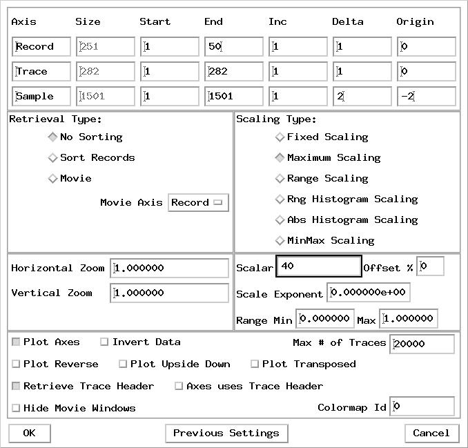